Previously, we introduced and explained different fairness algorithms that can be used to mitigate bias in a dataset or model predictions. Here, we will discuss a common misconception: removing the protected attribute from the dataset will remove bias. We show why this is not the case and why it is essential to use fairness algorithms.

Hiding Protected Attribute:

Our setup is the following: we have two workflows, and both are using the adult data set. In the first workflow, we will train a logistic regression model using Reweighing as a preprocessor and a regular logistic regression model as a baseline on data that has not been modified. The second workflow uses the same dataset but with the protected attribute removed. We will then compare the predictions of the two workflows using a Box Plot.

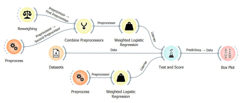
The two workflows are very similar, the only difference being the extra learner used in the first workflow, the reweighted learner, and two Select Columns widgets used in the second workflow. The first Select Columns widget is used to remove the protected attribute from the data, and the second one is used to add it back after the predictions are made so that we can compare the predictions of the two workflows using a Box Plot widget.

In this example, we will not be able to use the scores to compare the fairness metrics of the models because we could not calculate the fairness metrics for the workflow with the hidden protected attribute. This is because the protected attribute is required to calculate the fairness metrics. Saying that we can still compare the accuracy scores of the models. Here are the scores for the reweighted model, the baseline model, and the model learning on altered data:

The baseline model and the model learning on altered data have very similar accuracy scores, while the reweighted model has a slight dip in accuracy.

Instead of using the scores to compare the models, we will visualize the fairness Disparate Impact and Statistical Parity Difference fairness metrics using the Box Plot widget, just like we did in many previous blogs. Here we will show three different box plots, the first one will be from the reweighted model, the second one from the baseline, and the third from the model learning on data with the protected attribute removed:

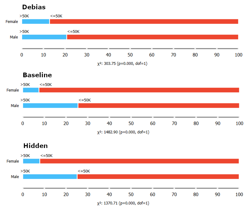
The box plots show that the baseline model results are very similar to the model learning on data with the protected attribute removed. In contrast, the reweighted model results are very different. The ratio of favorable prediction is much more similar when using debiasing compared to the baseline model and the model learning on data with the protected attribute removed.

A similar observation can be made for the Equalized Odds Difference and Average Odds Difference fairness metrics. Using a similar setup as in the previous blog post, we visualized the True Positive Rate for each group using the mosaic display widget. We trained one model using the Equalized Odds Postprocessing widget and one on data with the protected attribute “age” hidden. Here are the results:

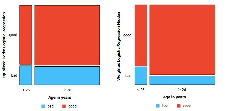
In the visualizations, the red part of each column represents the true positive rate for each group; you can ignore the width of the columns as that represents the number of instances in each group, which is irrelevant to us. We can see that the difference in True Positive Rate between the two groups is much smaller when using the Equal Odds Postprocessing widget.

Why and how?

If we removed the protected attribute from the dataset on which we train and test the model, how is it that the predictions are still biased towards one of the groups?

The answer is that features in a dataset are often correlated. This means that even if we remove the protected attribute, other features can still be used to infer the protected attribute. For example, suppose the protected attribute is race, and we have a feature like zip code in the data. Since certain races might be predominant in particular zip codes, the model may still indirectly learn the bias. We can test this correlation by predicting the protected attribute from the other features. If we can predict the protected attribute with high accuracy, we know that the other features are correlated with the protected attribute. Here is an example of such a workflow:

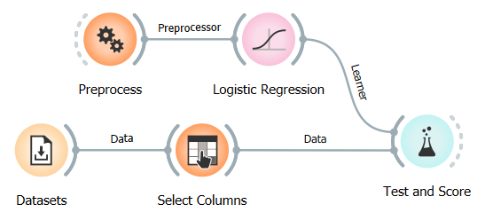
In this workflow, we set the “sex” attribute as the target variable and use a Logistic Regression model to try and predict it.

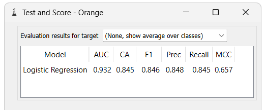
We can see that the model has a very high accuracy score, which means that the other features in the dataset are correlated with the protected attribute. This means that even if we remove the protected attribute from the dataset, the model can still infer it from the other features. This is why it is crucial to use fairness algorithms instead of simply removing the protected attribute.