Our recent project with the Ministry of Public Administration comprises building a semantic analysis pipeline in Orange, enabling the users to quickly and efficiently explore the content of documents, compare a subset against the corpus, extract keywords, and semantically explore document maps. If this sounds too vague, don’t worry, here’s a quick demo on how to perform semantic analysis in Orange.

First, we will use the pre-prepared corpus of proposals to the government, which you can download here. These are the initiatives which the citizens of Slovenia propose to the current government for consideration. The present corpus contains 1093 such proposals.

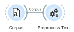
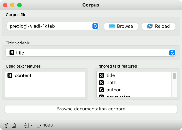
Each proposal contains a title, the content of the proposal, the author, the date when it was published, number of upvotes, and so on. But for a thousand proposals, it would take a long time to read all of them and see which policy areas they cover. Instead, we will use two new Orange widgets to determine the content (main keywords) of a subset of documents.

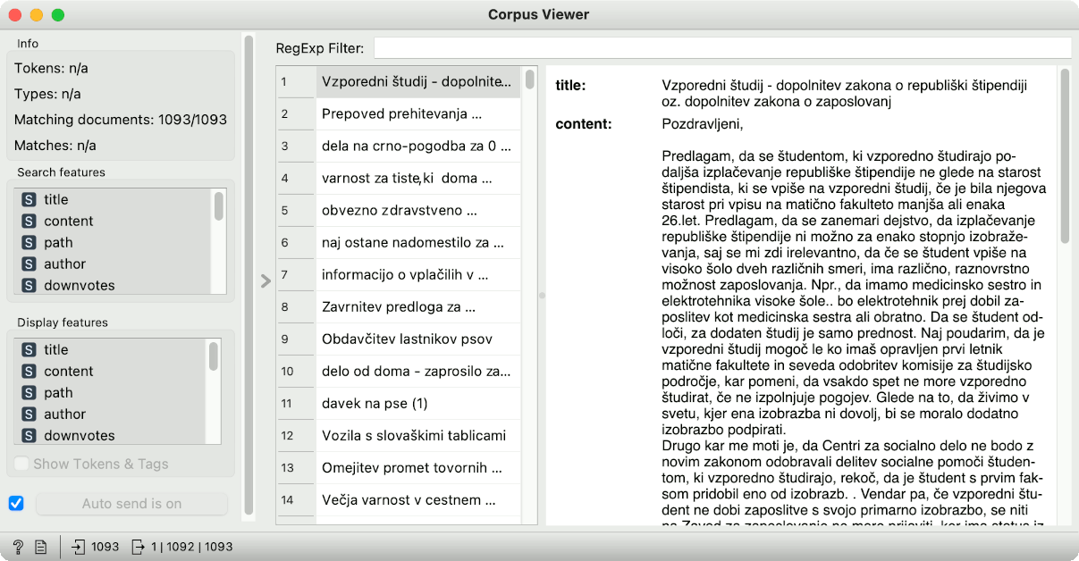
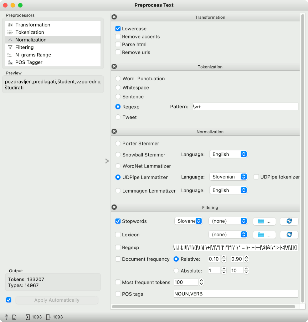
As always, we will first preprocess the corpus to create tokens, the core units of our analysis. The preprocessing pipeline is sequential; first, we lowercase the text, then we split the text into words (this is what the regular expression \w+. does), transform the words into lemmas with UDPipe, and finally remove stopwords from the list (such as “in”, “da”, “če”). Since we are working with a Slovenian language text, we have to select the corresponding models and stopword lists.

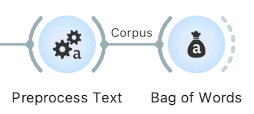
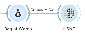
After preprocessing, we build a document-term matrix using the Bag of Words widget with the Count+IDF setting. Next, we pass the data to t-SNE to observe the document map. t-SNE takes the document-term matrix and finds a 2D projection, where similar documents lie close together.

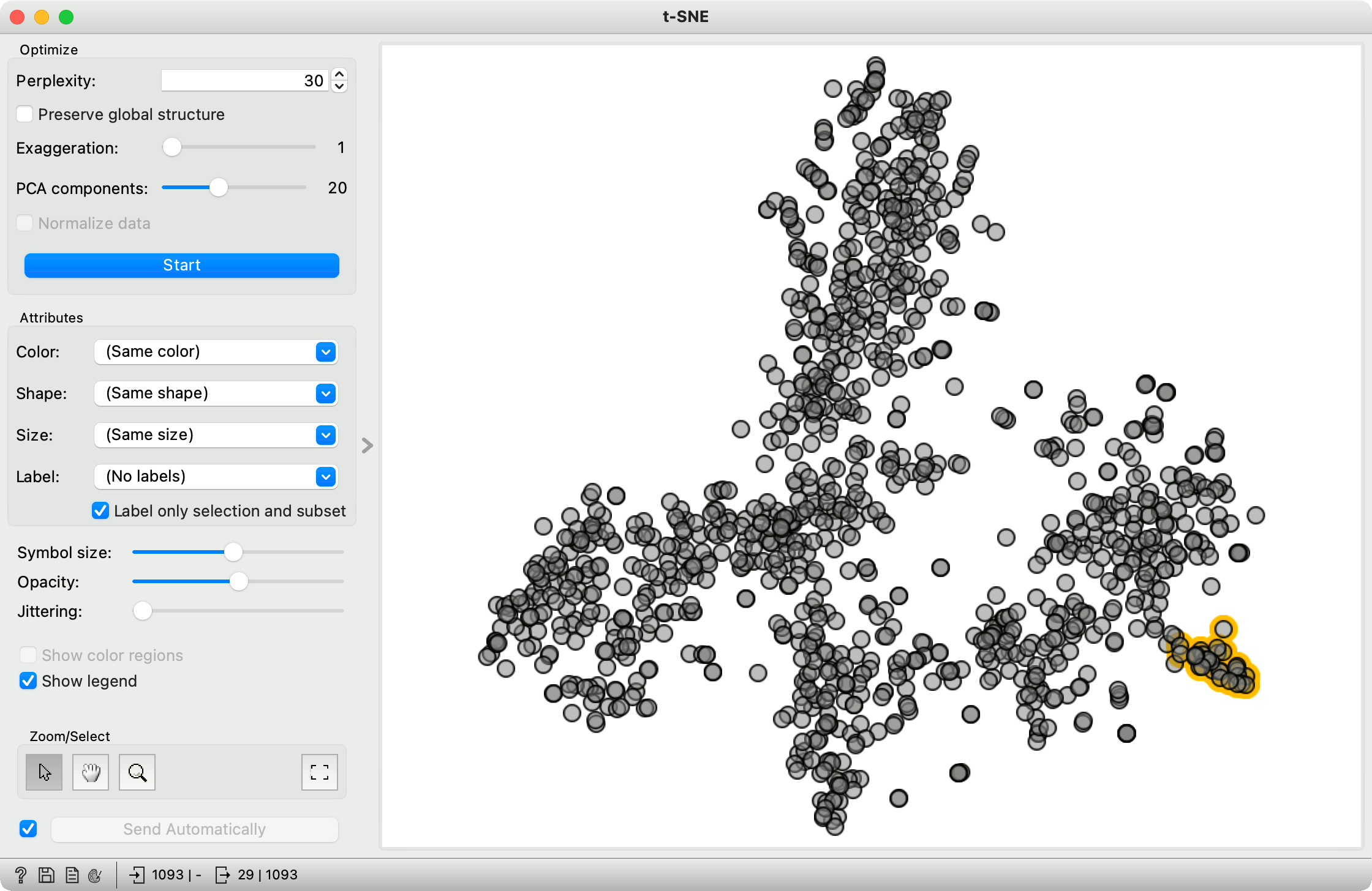
Now we will select a small subset of the document, say in the lower right corner, where we have a nice cluster of points. The question is, what are these documents talking about?

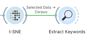
We will use Extract Keywords widget to find the most significant keywords in the selection. There are several methods we can use, even the popuar YAKE!, but we will go with a simple TF-IDF method, which takes the words with the highest TF-IDF score. Note that the vectorizer uses the default sklearn’s TfidfVectorizer settings, that is the tf-idf transform with L2 norm, keeping the passed tokens as they are.

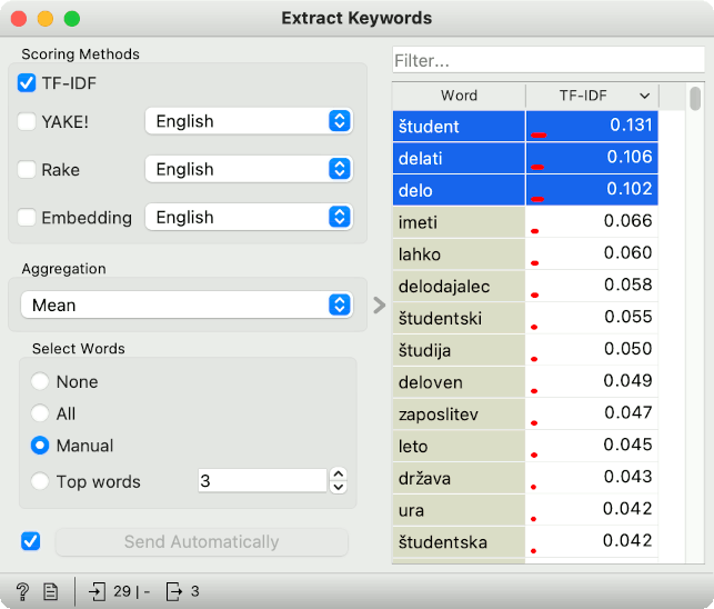
It looks like the top words characterizing the selected subcorpus are “študent” (student), “delati” (to work), and “delo” (the work). Apparently, the documents talk mostly about student work. Let us explore this a bit further. It would be nice to have a certain score attached to the documents, which would correspond to how much a document talks about student work. In other words, we would like to score the documents based on how many of the selected words they contain (and in what proportion).

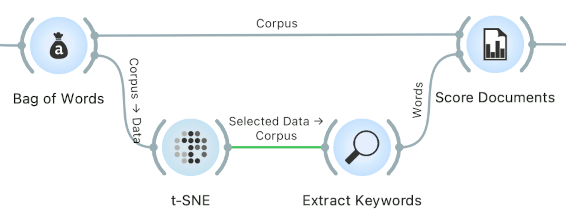
To achieve this, we will use Score Documents. We will pass it the document-term matrix and the list of selected keywords from Extract Keywords. The widget again offers several different ways of scoring documents. A simple way to score them is to compute how often selected words appear in each document, which corresponds to the “Word Count” method.

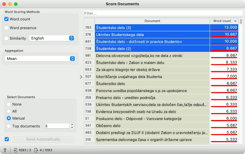
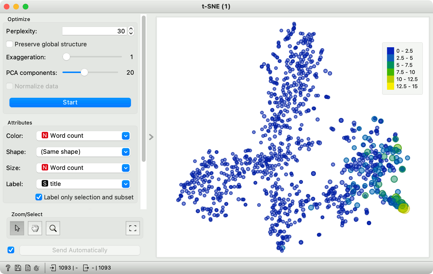
Score Documents returns keyword scores for each document. Let us pass the scored documents to another t-SNE widget. If we set the color and the size of the points to “Word Count” variable, t-SNE plot will expose the documents with the highest scores. These documents talk the most about students and work. A great thing is that we can see documents with high scores that were not a part of our selection, which means the general bottom-right area contains documents relating to this topic.

Now try selecting a different subset yourself and see what the documents are about. You can use any corpus you want, even the ones that come with Orange.