There have recently been some additions to the lineup of Orange learners. One of these is Orange.regression.earth.EarthLearner. It is an Orange interface to the Earth library written by Stephen Milborrow implementing Multivariate adaptive regression splines.

So lets take it out for a spin on a simple toy dataset (data.tab - created using the Paint Data widget in the Orange Canvas):

import Orange
from Orange.regression import earth
import numpy
from matplotlib import pylab as pl

data = Orange.data.Table("data.tab")
earth_predictor = earth.EarthLearner(data)

X, Y = data.to_numpy("A/C")

pl.plot(X, Y, ".r")

linspace = numpy.linspace(min(X), max(X), 20)
predictions = [earth_predictor([s, "?"]) for s in linspace]

pl.plot(linspace, predictions, "-b")
pl.show()

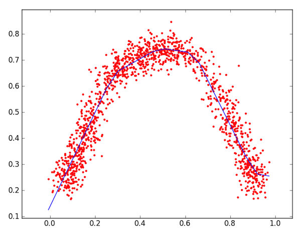
which produces the following plot:

We can also print the model representation using

print earth_predictor

which outputs:

Y =
   1.013
   +1.198 * max(0, X - 0.485)
   -1.803 * max(0, 0.485 - X)
   -1.321 * max(0, X - 0.283)
   -1.609 * max(0, X - 0.640)
   +1.591 * max(0, X - 0.907)

See Orange.regression.earth reference for full documentation.

(Edit: Added link to the dataset file)